Statistics of Weather and Climate Extremes

Background
Purpose This web page is intended to serve as a resource for the use of the statistical theory of extreme values in the analysis of weather and climate extremes and their impacts. It also serves as a gateway to the Extremes Toolkit. It was originally developed in conjunction with NCAR's Weather and Climate Impact Assessment Science Program, concerned with improving the scientific basis of assessments of the impacts of weather and climate on society (e.g., those of the U.N. Intergovernmental Panel on Climate Change, IPCC).
Statistical Theory of Extreme Values
(1) Block Maxima This theory has been well developed for quite a while. One important theorem states that the maximum of a sequence of observations, under very general conditions, is approximately distributed as the generalized extreme value (GEV) distribution. This distribution has three types (click on image below to enlarge):
(i) Gumbel A distribution with a light upper tail and positively skewed. (ii) Frechet A distribution with a heavy upper tail and infinite higher order moments. (iii) Weibull A distribution with a bounded upper tail.
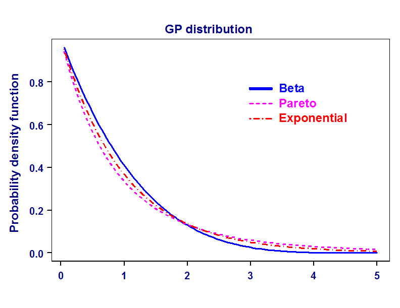
(2) Peaks Over Threshold In terms of the tail of a distribution, the corresponding theorem states that the observations exceeding a high threshold, under very general conditions, are approximately distributed as the generalized Pareto (GP) distribution. This distribution has three types (click on image below to enlarge):
(i) Exponential A light-tailed distribution with a "memoryless" property. (ii) Pareto A heavy-tailed distribution (sometimes called "power law"). (iii) Beta A bounded distribution.
The modern approach to extreme value analysis is based on a point process representation, equivalent to: (i) a Poisson process governing the rate of occurrence of exceedance of a high threshold; and (ii) a generalized Pareto distribution for the excess over the threshold. Through a reflection principle, the above theory can be converted into an equivalent form when the maximum is replaced by the minimum or an upper tail by a lower tail.
(3) Penultimate Approximations Use of a specific type of GEV or GP distribution can be thought of as an "ultimate" approximation. In practice, it is nearly always preferable to make use of the general form of GEV or GP distribution (which include the three types as special cases). This approach takes advantage of what is known as a "penultimate" (or more refined) approximation. For example, when maxima are obtained from normally distributed variables, the ultimate approximation is the Gumbel type of GEV distribution. Yet the Weibull type of GEV would provide a more accurate approximation.
(4) Clustering at High Levels
In the block maxima approach, the GEV approximation still holds under temporal dependence of extremes, but with effects on the center and spread of the distribution. In the peaks over threshold approach, temporal dependence of extremes can be circumvented through "declustering," in which only the single highest value (or cluster maximum) is retained from a run of consecutive values exceeding a high threshold.
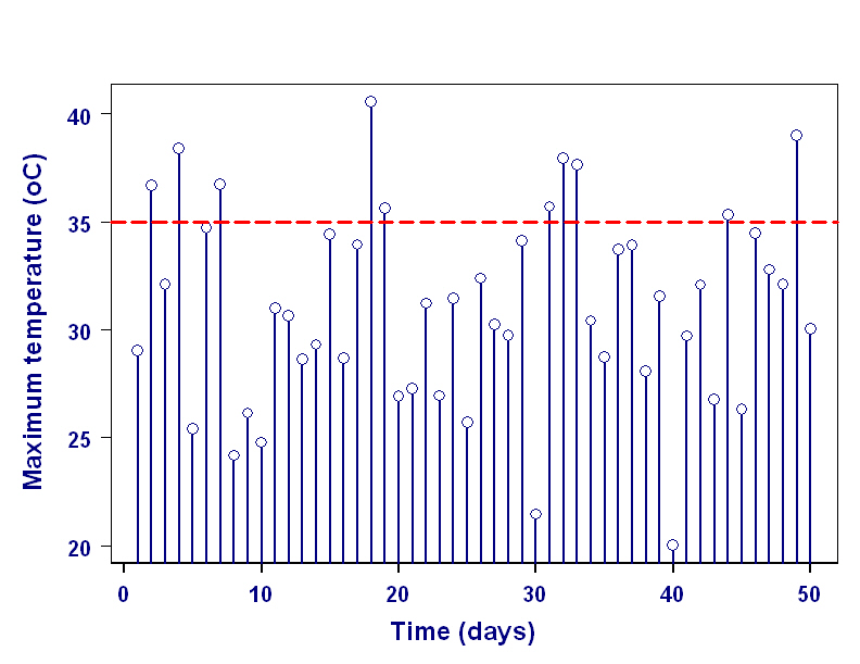
Weather and Climate Extremes With the computational advances and software developed in recent years, the application of the statistical theory of extreme values to weather and climate has become relatively straightforward. Annual and diurnal cycles, trends (e.g., reflecting climate change), and physically-based covariates (e.g., El Nino events) all can be incorporated in a straightforward manner. Consistent with the point process representation, the "peaks over threshold" (or "partial duration series") approach enables the use of more of the information available about the upper tail of the distribution (e.g., not just the annual maxima).
Return Levels and Return Periods
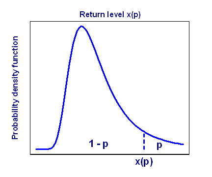
The concepts of return level and return period are commonly used to convey information about the likelihood of rare events such as floods. A return level with a return period of T = 1/p years is a high threshold x(p) (e.g., annual peak flow of a river) whose probability of exceedance is p. For example, if p = 0.01, then the return period is T = 100 years. Two common interpretations of a return level with a return period of T years are:
(i) Waiting time: Average waiting time until next occurrence of event is T years (ii) Number of events: Average number of events occurring within a T-year time period is one

Home | History | Links | Quotes | References | Software| Toolkit